All published articles of this journal are available on ScienceDirect.

A Comparative Study of ARIMA, ARFIMA and ARIMA-ARFIMA Models in Predicting Under-five Mortality Rate in Four East-African Nations
Abstract
Introduction
Despite significant advancements over the previous three decades, under-five mortality is still a significant public health concern in East Africa. Sustainable Development Goal (SDG) 3.2 calls for a reduction in under-five mortality to 25 deaths per 1,000 live births by 2030. Recent evaluations show that the area is not on course to attain the SDG objective, despite considerable declines in Kenya, Rwanda, Tanzania, and Uganda. This study compares the forecasting performance of Autoregressive Integrated Moving Average (ARIMA), Autoregressive Frictionally Integrated Moving Average (ARFIMA), and hybrid models for predicting under-five mortality rates (U5MR) in four East African countries and assesses their projected progress toward SDG 3.2.
Methods
Annual U5MR data for 1995–2022 were obtained from the World Bank. Differencing was used to attain stationarity after initial Augmented Dickey-Fuller (ADF) tests revealed non-stationarity in all four nations. ARIMA, ARFIMA, and hybrid models tailored to each country were fitted and assessed using AIC, BIC, RMSE, MAE, MAPE, and R2. The Ljung-Box test was used to determine residual independence. The best-performing models were used to create forecasts for 2023 to 2030.
Results
In every country, ARIMA models performed better than ARFIMA and hybrid models, exhibiting the best residual diagnostics and the lowest error metrics. Through 2030, U5MR is expected to continue declining, although none of the four nations are expected to meet the SDG 3.2 objective.
Discussion
To achieve SDG 3.2 in East Africa, child survival initiatives and healthcare systems must be strengthened.
Conclusion
In every country, ARIMA models performed better than other models, showing the best residual diagnostics and the lowest error metrics. Although U5MR is expected to continue declining through 2030, none of the four nations is expected to meet the SDG 3.2 objective.
1. INTRODUCTION
Sustainable Development Goal (SDG) 3.2, which seeks to lower under-five mortality to 25 deaths per 1,000 live births by 2030, places a strong emphasis on reducing under-five mortality [1]. Due to enduring socioeconomic disparities, health system constraints, and unequal access to high-impact child health interventions, East Africa continues to see slight decreases than the rest of the world despite advances [2-4].
In 2023, the UN Inter-agency Group for Child Mortality Estimation (UN IGME) reported a global under-five mortality rate (U5MR) of roughly 37 deaths per 1,000 live births [2, 3]. In sub-Saharan Africa, the U5MR remains about 68 deaths per 1,000 live births, according to the most recent data [1]. While recent data for Kenya, Rwanda, Tanzania, and Uganda differ, several national estimates indicate Uganda's U5MR at 39 per 1,000 live births, which is still significantly higher than the SDG 3.2 target of 25 per 1,000 [5]. These results show that, while significant reductions have been made throughout the area, the rate of decline has slowed in the SDG era, with global yearly reductions falling from approximately 3.7% in 2000-2015 to 2.2% in 2015-2023 [1, 3].
Time-series approaches, such as the Autoregressive Integrated Moving Average (ARIMA) model, are commonly used to model and forecast health indicators because they successfully capture short-term autocorrelation and linear temporal structure [6]. For series with long-memory or slow-decaying correlations, the Autoregressive Fractionally Integrated Moving Average (ARFIMA) model may provide better performance via fractional differencing. Hybrid techniques that incorporate ARIMA and ARFIMA have also received attention for capturing both short- and long-term memory properties [7, 8].
However, few studies have evaluated ARIMA, ARFIMA, and hybrid models for forecasting under-five mortality in East Africa. Understanding the most accurate forecasting strategy is critical to helping the region's progress towards SDG 3.2. This study examines and evaluates the forecasting effectiveness of ARIMA, ARFIMA, and hybrid ARIMA-ARFIMA models for Kenya, Rwanda, Tanzania, and Uganda using panel data from 1995 to 2022.
2. METHOD AND MATERIALS
2.1. Data Source
Using annual time-series data from Kenya, Rwanda, Tanzania, and Uganda, we analysed under-five mortality rates per 1,000 live births. Statistics from 1995-2022 were gathered from the World Bank's web-based development indicators catalogue. This balanced panel of four countries (with data from 1995-2022) allows for consistent comparisons between them across time. Data series from each country were examined using time-series models. To assess the effectiveness of univariate time series forecasting on mortality rate trajectories, no further exogenous factors were added. U5MR is defined as the number of deaths among children under five per 1,000 live births.
2.2. Study Variables
This study measures the UFMR, which is the number of deaths in children under five (U5D) per 1,000 live births each year. Our goal is to anticipate the rate (dependent variable). These models are univariate, relying solely on historical U5MR values to predict future values. The models use time (measured in years) as the independent variable to capture temporal patterns and trends in the under-five mortality rate from 1995 to 2022. No other factors are utilised in these models, aligning with the focus on mortality rate time-series behaviour.
2.3. Stationarity and Time Series Modelling Approach
2.3.1. Stationarity
Prior to modelling, the stationarity properties of the under-five mortality series were evaluated using the Augmented Dickey-Fuller (ADF) test, which determines if a time series has a unit root, indicating non-stationarity. The ADF test relies on the following regression in Eq. (1):
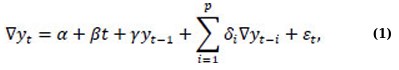
where, yt is the time series value, ∇yt = yt - yt-1 represents first differencing, t is the time trend, γ is the coefficient used to test for a unit root, p is the number of lagged difference term added to remove autocorrelation, and εt is a white noise. The hypothesis tested is
H0: the series has a unit root (non-stationary).
Ha: the series is stationary.
If the ADF test statistic is more negative than the critical value, or if the p-value is > 0.05, the null hypothesis is rejected, showing stationary behaviour. If not, the series is deemed non-stationary, and differencing is required to stabilise the mean and variance. Also, detrending and Box-Cox transformation may be applied. Stationarity is required for ARIMA and ARFIMA models because non-stationary data can produce biased parameter estimates and incorrect forecasts.
2.3.2. Autoregressive Integrated Moving Average
The ARIMA method delineates the linear trends and short-term variations in the under-five mortality rate series for each nation [7]. Stationary time series data or data that has been rendered stationary through differencing demonstrates robust performance [7, 9, 10]. The ARIMA model is characterised by three parameters: p, representing the number of autoregressive (AR) terms; d, indicating the degree of differencing; and q, denoting the number of moving average (MA) terms [11, 12]. An ARIMA model is defined as Eq. (2):

where ϕB and θB denotes polynomials in the backshift operator B.
2.3.3. Autoregressive Fractionally Integrated Moving Average
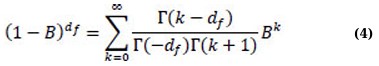
The ARFIMA model is employed in mortality data to identify long-memory characteristics and trends that ARIMA models may struggle to detect [7, 12]. The extent of long-range dependence is assessed by measuring the fractional differencing parameter [12, 13]. This is beneficial in contexts such as health data, where autocorrelations in the data progressively decline over time [14, 15]. The ARFIMA model is characterized by three parameters: p, representing the number of autoregressive (AR) terms; df , indicating the degree of frictional differencing; and q, denoting the number of moving average (MA) terms. An ARFIMA model is defined as Eq. (3):

with the frictional differencing operator given by the binomial expansion (Eq. 4):
2.3.4. ARIMA-ARFIMA Hybrid Model
The hybrid model improves prediction accuracy by combining the long-memory attributes of ARFIMA with the short-memory structure of ARIMA [7]. This study's hybrid model amalgamates forecasts from the ARIMA and ARFIMA models, capitalising on the advantages of both methodologies. Following the classical residual-modelling strategy (Eqs. 5 and 6):
Step 1: Fit ARIMA to the original series, yt
Step 2: Extract residuals:
Step 3: Fit an ARFIMA model to the ARIMA residuals to capture long-memory structure.
Step 4: Combine forecasts:
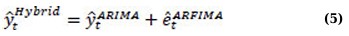
This framework facilitates the integration of ARIMA's predictive capabilities for short-term trends with ARFIMA's capacity for long-term dependencies.
2.4. Model Selection and Parameter Optimisation
2.4.1. Model Selection
Model selection in time-series analysis is choosing the best structure to capture the stochastic patterns found in a dataset. For ARIMA-type models, this method entails determining the best autoregressive order (p), differencing order (d), and moving-average order (q) [7]. Selection is frequently guided by information criteria such as the Akaike Information Criterion (AIC), corrected AIC (AICc), and Bayesian Information Criterion (BIC), which discourage excessive parameterisation while rewarding improved fit [16]. AIC value is given by Eq. (6):

where, k represents the number of parameters and L represents the likelihood. In contrast to the Akaike Information Criterion (AIC), the Bayesian Information Criterion (BIC) imposes a more stringent penalty on model complexity; lower values signify a superior fit [16, 17]. BIC value is given by Eq. (7):

where n represents the quantity of observations. In the process of model selection, AIC and BIC are calculated to determine the most suitable parameter combinations [17]. Lower information-criterion values suggest better-suited models. Automated techniques, such as the auto.arima (in R software version 3.6.3) algorithm, is frequently used in time-series modelling nowadays. Auto.arima searches systematically across a wide range of p, d, and q values, uses unit-root tests to identify acceptable differencing, and assesses candidate models using AICc or BIC [16]. It also checks for stationarity and invertibility restrictions, as well as seasonal components where applicable. This automated methodology promotes efficiency and model parsimony while offering a data-driven foundation for selecting well-specified ARIMA models [18, 19]. When selecting ARFIMA models, it's important to choose fractional differencing parameters that are stationary and invertible within the range of -0.5 to 0.5 [7]. Hybrid modelling approaches often begin by selecting the best ARIMA and ARFIMA models separately before assessing the value of merging their projections [20].
2.4.2. Parameter Estimation
Maximum likelihood estimation (MLE) is commonly used to estimate parameters in ARIMA, ARFIMA, and hybrid models. In ARIMA models, MLE is used to estimate the autoregressive and moving-average parameters by maximising the observed series' likelihood under the assumed model [21]. The differencing order d assures stationarity, whilst the calculated coefficients must adhere to theoretical restrictions that ensure the model's stationarity and invertibility [21].
2.4.3. Model Diagnostics and Validation
For ARFIMA models, MLE also estimates the fractional differencing parameter, allowing the model to reflect long-memory features. The parameter estimate technique ensures that the fractional differencing value is within the feasible range, which maintains model stability. Hybrid model parameter estimation normally entails estimating each component model individually and then establishing combination weights, which are frequently chosen to minimise forecasting error metrics such as the Root Mean Squared Error (RMSE). MLE produces consistent and efficient parameter estimations across model classes when the underlying assumptions are met. Estimated parameters must be statistically significant, theoretically sound, and supported by diagnostic tests [21]. Model diagnostics are required to ensure that the selected and estimated model accurately captures the underlying data-generation process. Diagnostic evaluation is primarily concerned with the behaviour of model residuals [22]. A correctly stated model should produce residuals that look like white noise, such as uncorrelated, random, and with constant variance [22]. Residual independence is typically evaluated using the Ljung–Box Q-test, which tests the null hypothesis that model residuals exhibit no autocorrelation [22]. The following provides the test statistic (Eq. 8):
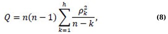
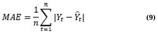
where ρk is the sample autocorrelation at lag k, n is the number of observations, h is the number of lags being tested, and Q is the Ljung-Box statistic. A non-significant p-value supports the adequacy of the fitted model [22]. Model adequacy is further assessed using forecast accuracy metrics, including Mean Absolute Error, Root Mean Square Error, Mean Absolute Percentage Error, and R2, to ensure that the model performs reliably in both fitting past observations and predicting future values [23]. The average magnitude of errors is quantified by the Mean Absolute Error, or MAE. The Mean Absolute Error diminishes as model accuracy improves. The optimal approach for understanding the overall average error is to utilize the same units as the original data [24]. It is given by Eq. (9):
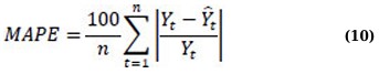
The Mean Absolute Percentage Error (MAPE) simplifies the comprehension of errors by representing them as percentages. Better forecasting accuracy is indicated by a lower MAPE [23, 24]. MAPE is given as follows in Eq. (10):
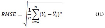
Root Mean Square Error (RMSE) penalises large errors severely because of squaring [24]. Better performance is indicated by a lower RMSE [9, 22, 23], and given by Eq. (11):
Contextual judgement is used to determine whether outlier sensitivity or percentage error is more important when one metric is inconsistent (such as one model has a lower MAE but a higher RMSE) [23, 25].
3. RESULTS
3.1. Exploratory Data Analysis
Figure 1a-d indicate that under-five mortality rates decreased significantly in all four East African countries between 1995 and 2022, albeit the amount of reduction varied by country. Kenya has had a continuous and constant drop, from more than 110 fatalities per 1,000 live births in the mid-1990s to around 41 deaths per 1,000 in 2022. Rwanda has shown the most dramatic improvement, with mortality dropping from more than 220 deaths per 1,000 live births in 1995 to around 38 deaths per 1,000 in 2022, owing primarily to faster increases between 2000 and 2010. Tanzania also shows a smooth and steady decline, falling from approximately 160 to 42 deaths per 1,000 during the timeframe, while Uganda follows a similar downward pattern, falling from around 165 to 40 deaths per 1,000. Overall, the four panels show persistent improvements in child survival across the region; however, despite these gains, none of the countries have yet met the SDG 3.2 target of 25 deaths per 1,000 live births, highlighting the need for further strengthening of child health measures.
3.2. Stationarity Test
Initial Augmented Dickey-Fuller (ADF) tests on the raw under-five mortality series for Kenya, Rwanda, Tanzania, and Uganda revealed that all four countries exhibited non-stationary data with p-values greater than 0.05, indicating the presence of unit roots. As a result, differencing was applied to each country's series, and a column in the results table indicates the number of differences needed to ensure stationarity for each dataset. After differing twice, the ADF tests were redone, and Table 1 displays the resulting ADF statistics and p-values for the four countries. All examples had p-values < 0.005, supporting the alternative hypothesis and rejecting the unit-root null. Rwanda and Uganda, for example, with the ADF statistics of -18.51 (p = 0.0001) and -7.92 (p = 0.0005), respectively, but Kenya and Tanzania also show high indications of stationarity. These findings demonstrate that, following proper differencing, the under-five mortality series from 1995 to 2022 are stationary at the 5% level.
3.3. Model Selection
Table 2 summarises the ARIMA model orders chosen for Kenya, Rwanda, Tanzania, and Uganda, together with their respective AIC and BIC values. After comparative examination revealed that ARIMA models were better suited to the current data than ARFIMA or hybrid alternatives, the auto.arima method was used to determine the best specification for each country. Auto.arima runs through multiple combinations of p, d, and q values, uses unit-root testing to guide differencing, and selects models with the lowest information-criterion values. For Kenya, the technique used ARIMA (0,2,1), which had an AIC of 42.77 and a BIC of 45.29. Rwanda and Uganda both chose ARIMA (1,2,0) as their best models, demonstrating relatively simple autoregressive structures after differencing. Tanzania required a more sophisticated autoregressive component, with ARIMA (4,2,0) providing the best results (AIC = 32.10; BIC = 38.39). Overall, the chosen models offer the most statistically efficient and concise ARIMA specifications for the differenced series, proving ARIMA's usefulness for modelling and forecasting under-five mortality in the four nations.
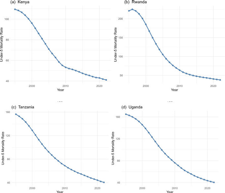
Trend plot of under-five mortality rates (UFMR) for Kenya, Rwanda, Tanzania, and Uganda, illustrating the historical changes in mortality rates from 1995 to 2022.
3.4. Model Performance Comparison
Table 3 summarizes the training and testing accuracy metrics for the selected ARIMA models, which were trained with 80% of the time-series data and tested with 20%. Across the training set, all four models had reasonably low MAE, RMSE, and MAPE values, indicating strong in-sample fitting. Kenya's ARIMA (0,2,1) achieved reasonable accuracy (MAE = 0.37; RMSE = 0.46), whereas Rwanda's ARIMA (2,1,0) generated more training errors (MAE = 0.79; RMSE = 1.12), indicating greater variability in its historical pattern. Tanzania's ARIMA (4,2,0) and Uganda's ARIMA (2,1,0) produced the best in-sample results, with low MAE and RMSE values (MAE ≈ 0.23-0.24; RMSE ≈ 0.27-0.29) that closely matched the actual data. In contrast, the test-set (20%) findings show higher variability in out-of-sample predicting performance. Kenya and Tanzania exhibit reasonably steady generalization, with moderate gains in MAE and RMSE (Kenya MAE = 0.52; Tanzania MAE = 0.59), showing that their ARIMA models maintained respectable predictive accuracy after training. However, Rwanda and Uganda show significant declines in forecast performance, particularly in MAPE, with Rwanda achieving a Test MAPE of 746.17 and Uganda 1671.98. These substantial out-of-sample errors point to increased structural fluctuations or anomalies in the latter stages of their time series. Overall, Tanzania's ARIMA (4,2,0) model generalises the best under the 80/20 split, while Rwanda and Uganda have worse predictive stability despite good in-sample performance.
| Country | ADF Statistic | p-value | Stationary | Differencing |
|---|---|---|---|---|
| Kenya | -3.76 | 0.0033 | Yes | 2 |
| Rwanda | -18.51 | 0.0001 | Yes | 2 |
| Tanzania | -5.88 | 0.001 | Yes | 2 |
| Uganda | -7.92 | 0.0005 | Yes | 2 |
| Country | ARIMA (p, d, q) | AIC | BIC |
|---|---|---|---|
| Kenya | (0, 2, 1) | 42.77 | 45.29 |
| Rwanda | (1, 2, 0) | 85.59 | 88.11 |
| Tanzania | (4, 2,0) | 32.10 | 38.39 |
| Uganda | (1, 2,0) | 22.71 | 25.26 |
| Country | Train_MAE | Train_RMSE | Train_MAPE | Test_MAE | Test_RMSE | Test_MAPE |
|---|---|---|---|---|---|---|
| Kenya | 0.37 | 0.46 | 58.72 | 0.52 | 0.56 | 121.85 |
| Rwanda | 0.79 | 1.12 | 74.42 | 2.94 | 3.80 | 746.17 |
| Tanzania | 0.23 | 0.27 | 27.57 | 0.59 | 0.72 | 133.13 |
| Uganda | 0.24 | 0.29 | 28.47 | 7.11 | 8.76 | 1671.98 |
Table 4 shows model fit statistics for the four countries' ARIMA models, including estimated error variance σ2, log-likelihood (LogLik), and AIC and BIC values. Kenya's ARIMA (0,2,1) model has a small error variance (σ2= 0.27) and a LogLik of -19.39, indicating a reasonable fit for a second-differenced series. Rwanda's ARIMA (1,2,0) has the highest error variance (σ2= 1.26) and lowest LogLik (-40.80), indicating higher variability and lower model fit compared to other countries. Tanzania's ARIMA (4,2,0) model has a low error variance (σ2= 0.15) and larger LogLik (-11.05). This, combined with a low AIC (32.10) and BIC (38.39), shows that the model captures the underlying dynamics more effectively despite having more parameters. Uganda's ARIMA (1,2,0) has the lowest error variance (σ2= 0.12) and a high log-likelihood (-9.37), resulting in the lowest AIC (22.74) and BIC (25.26) among all countries. Overall, these findings show that, while all four ARIMA models produce statistically adequate fits, Tanzania and Uganda have the highest overall model performance, whereas Rwanda has the weakest due to larger error variance and lower likelihood.
3.5. Residual Diagnostics
Table 5 shows the Ljung-Box test findings for the residuals of the selected ARIMA models across all four nations. The Ljung-Box statistic examines the null hypothesis, which states that the model residuals are independently distributed with no lingering autocorrelation. Across all nations, the p-values are considerably above the 5% significance threshold (Kenya: p = 0.6267; Rwanda: p = 0.9213; Tanzania: p = 0.9335; Uganda: p = 0.5421), indicating that the null hypothesis was not rejected. This result demonstrates that the residuals behave like white noise, indicating that the models accurately captured the autocorrelation structure in the differenced under-five mortality series. The consistently high p-values across all models show that there is no substantial serial dependency in the residuals, supporting the appropriateness of the selected ARIMA models for forecasting and indicating that no further model modification is necessary in terms of residual autocorrelation.
| Country | ARIMA Model | σ2 | LigLik | AIC | BIC |
|---|---|---|---|---|---|
| Kenya | (0, 2, 1) | 0.27 | -19.39 | 42.77 | 45.29 |
| Rwanda | (1, 2, 0) | 1.26 | -40.80 | 85.59 | 88.11 |
| Tanzania | (4, 2,0) | 0.15 | -11.05 | 32.10 | 38.39 |
| Uganda | (1, 2,0) | 0.122 | -9.37 | 22.71 | 25.26 |
| Country | ARIMA Model | Q statistic | P-value |
|---|---|---|---|
| Kenya | (0,2,1) | 8.022 | 0.627 |
| Rwanda | (1,2,0) | 4.512 | 0.921 |
| Tanzania | (4,2,0) | 4.286 | 0.934 |
| Uganda | (1,2,0) | 8.895 | 0.542 |
3.6. Forecasting
Figure 2 shows ARIMA-based projections of under-five mortality rates for Kenya, Rwanda, Tanzania, and Uganda from 2023 to 2030, with historical values in solid black, anticipated values in dashed green lines, and 95% confidence intervals represented by shaded green regions. These ranges show the range within which future mortality estimates are projected to fall with 95% certainty, and they broaden with time as uncertainty increases as the model projects further beyond the observed data. The predictions for all four countries show persistent declines in under-five mortality; nevertheless, the predicted reductions are inadequate for any of the nations to meet the SDG 3.2 target of 25 deaths per 1,000 live births, as illustrated by the red dashed line. Kenya (Fig. 2a) exhibits a moderate declining trend but remains above the SDG criteria for the projection period. Rwanda (Fig. 2b), despite experiencing the highest historical fall, remains above the objective. Tanzania (Fig. 2c) shows significant gains, but the anticipated values remain above the SDG objective even after allowing for uncertainty. Uganda (Fig. 2d) is on a similar course, with mortality progressively declining but still expected to surpass the target by 2030. Overall, while improvements are predicted to continue, the projection intervals show that, even under the most optimistic scenarios, none of the four countries is expected to fulfil the SDG 3.2 under-five mortality target by 2030.
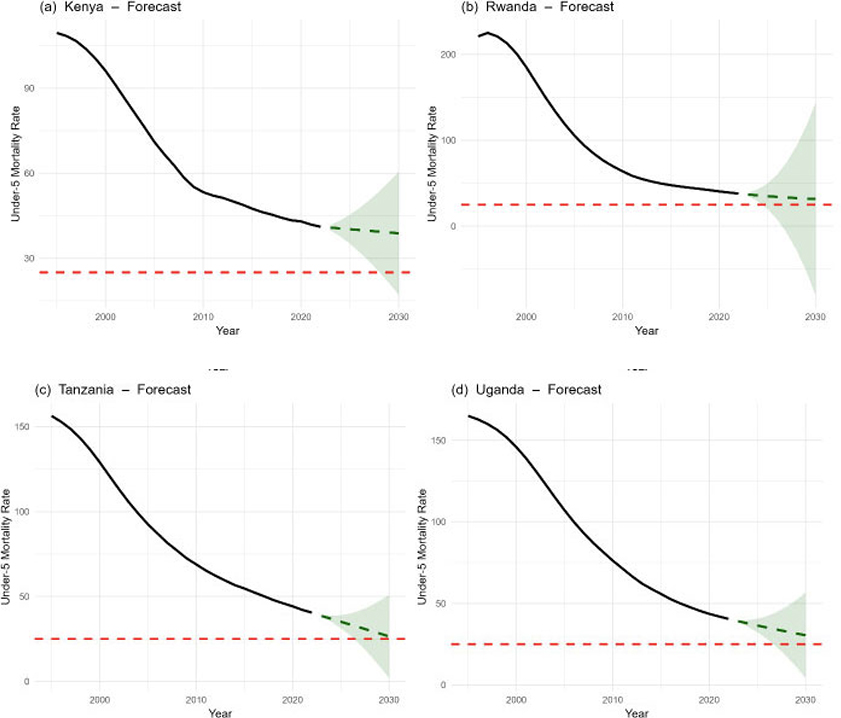
(a-d) Projection of under-five mortality rates (UFMR) for Kenya, Rwanda, Tanzania, and Uganda from 2023 to 2030, with SDG target (red line).
4. DISCUSSION
The findings of this analysis indicate considerable gains in reducing under-five mortality in Kenya, Rwanda, Tanzania, and Uganda from 1995 to 2022, consistent with advances in the region described by recent global assessments of child survival [1, 4]. All four countries display pronounced downward trends in the mortality rates over time, but at very different speeds. Rwanda made the fastest progress, which likely reflects very intense post-conflict health system strengthening, versus Kenya, Tanzania, and Uganda, where improvements they experienced have been more incremental. These differences reveal heterogeneity in the delivery and impact of interventions to improve child survival in East Africa, as observed elsewhere [26, 27]. The stationarity assessment provided a critical foundation for model development. The strong stationarity after differencing reflects the smooth long-term decline in U5MR and supports the appropriateness of ARIMA models for these series [12]. Differencing was therefore required to stabilise the mean, and the number of differences needed for each country was reported in the results table. Once differenced, the ADF tests indicated significant stationarity (all p < 0.005), confirming the suitability of ARIMA-type models for further analysis.
According to a comparison of modelling techniques, ARIMA models outperformed both ARFIMA and hybrid models for this dataset, which is consistent with the benefits of ARIMA for comparatively smooth, short-memory demographic processes that have been previously documented [6]. Although long-memory behaviour can be accommodated by ARFIMA models [8, 28], the current time series did not exhibit such persistent long memory reliance. Thus, ARIMA (0,2,1) for Kenya, ARIMA (1,2,0) for Rwanda and Uganda, and ARIMA (4,2,0) for Tanzania were obtained by using the arima algorithm for each nation using the estimation dataset to determine the optimal p, d, and q parameters. Other models are statistically efficient since their AIC and BIC values were higher. The suitability of the selected models is further supported by the ARIMA fit statistics. Rwanda was the least favoured, most likely because of structural volatility in its mortality series, while Tanzania and Uganda showed the highest log-likelihood values and the lowest estimated error variance. All models showed comparatively good in-sample performance, as evidenced by the low training MAE and RMSE values, according to performance evaluation using an 80/20 split. Out-of-sample performance, however, was inconsistent: Rwanda and Uganda experienced a notable increase in test-set errors, especially MAPE, which suggests that this could be caused by either local shocks or higher recent variability or structural breaks underpinning ARIMA models [29]. Kenya and Tanzania, on the other hand, had reasonable stability in predictions.
The overall suitability of the models' fit was confirmed by residual diagnostics. The Ljung-Box Q-test produced substantial p-values (all > 0.54), indicating that the ARIMA models sufficiently compensated for temporal dependence in the differenced series and supporting the lack of significant residual autocorrelation. These findings are consistent with the typical model adequacy standards for time series forecasting [30].
Forecasts for the years 2023 to 2030 indicate that under-five mortality will continue to decline in all four nations. However, the SDG 3.2 objective of 25 fatalities per 1,000 live births by 2030 is still exceeded by expected rates [1, 4, 31]. Not a single nation is predicted to meet the SDG objective within the prediction range, even with the strongest confidence interval limitations. This is in line with global data showing that several low- and middle-income nations are either already failing to meet their SDG objectives for child survival or are in danger of failing to do so [1, 4].
The results allow for the drawing of two key insights. The ARIMA models offer a reasonably solid and economical method for modelling and projecting under-5 mortality in East Africa; nevertheless, the accuracy of estimates depends on the stability of current data available for each country. Second, while significant improvement, the decline rate is insufficient to achieve SDG 3.2 by 2030; this indicates the need for more funding for health access, nutrition initiatives, vaccination coverage, and mother, newborn, and child health programs throughout the region.
The study has significant drawbacks. Annual national data were used, perhaps masking important subnational variances in child mortality. The univariate ARIMA models have little explanatory power due to their focus on healthcare access, immunisation, nutrition, and socioeconomic determinants [6]. Projections presume the past is prologue, thus any unexpected shock, such as a pandemic or war, could impact future outcomes. Large test-set MAPE for Rwanda and Uganda indicates a turbulent market, which ARIMA may not have fully captured [7]. Using secondary international datasets results in an estimated uncertainty [1]. Finally, multivariate or machine learning methodologies can enhance prediction performance for future investigations.
CONCLUSION
In this article, we have used ARIMA (p, d, q), ARFIMA (p, d, q), and a hybrid model to predict under-five mortality and have examined the long-term patterns of whether it is increasing, decreasing, or stable in all the countries. According to the study's findings, all four nations significantly reduced U5mr between 1995 and 2022, which is consistent with regional accomplishments reported in previous reports on global child survival [1, 4, 31]. Despite this progress, the first ADF tests of the data revealed that the raw mortality series were non-stationary, necessitating the differencing of these series before modelling. ARIMA outperformed ARFIMA and hybrid alternatives in terms of model fit, prediction accuracy, and residual diagnostics, making it the best modelling technique after second differencing.
For each of the four countries, ARIMA models consistently demonstrated excellent in-sample performance, passed every residual independence test recommended by Ljung-Box, and produced accurate projections between 2023 and 2030. Despite optimistic confidence ranges, the forecast estimates show that all countries are still not on track to meet the SDG 3.2 target of reducing under-five mortality to 25 deaths per 1,000 live births by 2030. These recent observations of high volatility are likely to continue, since Tanzania and Uganda show higher predictive trajectories, while Rwanda and Uganda show greater uncertainty.
These findings highlight progress made and ongoing efforts to reduce under-five mortality in eastern Africa. Key factors for sustainable progress include investment in primary healthcare systems, expansion of coverage to essential maternal and child health services, improvements in nutritional programs, and immunisation coverage; these need to be harnessed. Additionally, this work highlights the significance of employing robust time series models1 in health planning and recognises that more sophisticated multivariate or machine-learning techniques may continue to increase prediction accuracy.
AUTHORS’ CONTRIBUTIONS
The authors confirm their contribution to the paper as follows: W.J.D.: Analysis and interpretation of results; W.J.D., S.F.M., H.G.M.: Draft manuscript. All authors reviewed the results and approved the final version of the manuscript.
LIST OF ABBREVIATIONS
| SDG | = Sustainable Development Goal |
| ARIMA | = Autoregressive Integrated Moving Average |
| ARFIMA | = Autoregressive Frictionally Integrated Moving Average |
| U5MR | = Under-five mortality rates |
| ADF | = Augmented Dickey-Fuller |
| UN IGME | = UN Inter-agency Group for Child Mortality Estimation |
| AR | = Autoregressive |
| MA | = Moving average |
ETHICAL STATEMENT
The study is based on secondary analysis of publicly available, aggregated panel data obtained from the World Bank World Development Indicators database. The data do not contain individual-level or identifiable human or animal subject information; therefore, ethical approval was not required. The manuscript does not contain any individual-level identifiable data, personal details, biological samples, or audio-visual material. As such, informed consent was not applicable.
AVAILABILITY OF DATA AND MATERIALS
The data supporting the findings of this article are available from the World Bank World Development Indicators (WDI) database at https://databank.world bank.org/source/world-development-indicators. The panel data used in this study are publicly accessible and were retrieved directly from the World Bank Open Data repository.
CONFLICT OF INTEREST
Dr. Sileshi F. Melesse is in the Editorial Advisory Board Member of The Open Public Health Journal.
ACKNOWLEDGEMENTS
The authors thank the Department of Mathematical and Statistical Sciences at North-West University and the University of KwaZulu-Natal's School of Mathematics, Statistics, and Computer Science for providing support. They also thank the authors of the literature and the World Bank for providing access to the data needed for time series analysis and predicting under-five mortality.