All published articles of this journal are available on ScienceDirect.

Analysis of CD4 Count in People Living with HIV: An Additive Negative Binomial Mixed-effects Modeling of Longitudinal Data
Authors Info & Affiliations
Abstract
Introduction
CD4 cell counts provide insight into the health of a person’s immune system, as well as information about how their disease is progressing. Boosting the immune level of individuals living with HIV through antiretroviral medication is the most effective way to prevent complications and illnesses caused by Opportunistic Infections (OIs).
Methods
In this study, we conducted a longitudinal cohort analysis of CD4 count in people living with HIV using additive negative binomial mixed-effects models. A flexible Generalized Additive Mixed-effects Model (GAMM) framework was employed to capture complex nonlinear patterns in repeated CD4 measurements. The analysis was based on longitudinal data from the CAPRISA 002 Acute Infection (AI) study at the Centre for the AIDS Programme of Research in South Africa. Key variables, such as age, baseline BMI, and follow-up duration (time), were analyzed nonparametrically, along with other relevant factors analyzed parametrically.
Results
The study results revealed significant effects of baseline viral load and HAART initiation on CD4 count progression. Patients initiating HAART showed a 1.233-fold increase in expected CD4 count compared to pre-treatment levels. Baseline viral load negatively impacted CD4 count, even with small unit changes (γ =-1.581e-07, p-value=0.00079). Smooth terms of age (edf = 14.24, p-value < 2e-16), time (edf = 10.343, p-value < 2e-16), and baseline BMI (edf = 3.044, p-value = 2.21e-06) exhibited significant non-linear relationships with CD4 count. Spline plots indicated gradual CD4 improvement over time, suggesting long-term benefits of HAART, especially in older and higher-BMI patients.
Discussion
The findings of our analysis offer a deeper understanding of the functional relationship between the outcome variable and key predictors over time. The research found that initiating antiretroviral therapy improves trajectories of CD4 counts, whereas higher baseline viral load significantly impairs immune recovery over time. The modeling further revealed that age, time, and baseline BMI have a significant nonlinear impact on CD4 count dynamics over time.
Conclusion
The study establishes that BMI has an impact on the progression and immune responses of Highly Active Antiretroviral Therapy (HAART). The significant nonlinear effect of time suggests that the progress of patients’ CD4 count is slow, and higher CD4 count levels are observed after several treatment visits based on the studied data set. HIV patients who do not maintain immunological stability by consistently receiving antiretroviral medication face an increased risk of illness if they contract OIs due to weakened immune response.
1. INTRODUCTION
Human Immunodeficiency Virus (HIV), which causes Acquired Immune Deficiency Syndrome (AIDS), remains a major global health concern. Studies show that Sub-Saharan Africa bears the greatest share of the HIV/AIDS burden worldwide [1-3]. Despite numerous studies, articles, and discussions on HIV/AIDS, it remains a critical worldwide issue and a hindrance to progress. The impact of the HIV epidemic varies across regions worldwide, with Sub-Saharan Africa being the most affected region compared to other parts of the world [1-4]. The lessons learned from these regions are crucial for the global community [3-6]. While South Africa has one of the highest HIV prevalence globally, rising infection rates are also being observed across other regions, including parts of South and Southeast Asia, Latin America, Eastern Europe, Central and East Asia, the Middle East, and North Africa [3, 6].
According to the 2019 UNAIDS report, since the identification of the virus in 1983, over 70 million people have contracted HIV, and more than 40 million people have passed away due to AIDS-related causes around the world. Additionally, the report states that 7000 new infections are reported every day [1-5]. At the end of 2017, it was estimated that around 36.9 million people worldwide were living with HIV, with the range of the estimate being 31.1 to 43.9 million people. Although the percentage of adults aged 15-49 living with HIV was estimated to be around 0.8% [0.6-0.9%], there is still significant variation in the prevalence of the epidemic across different countries [7]. However, global endeavors to combat the pandemic are having a notable impact. Despite ongoing progress in HIV-related prevention strategies, clinical care, and therapeutic interventions, leading to a modest reduction in the annual incidence of HIV infections and mortality linked to AIDS, AIDS and its associated complications remain significant contributors to global mortality rates [1, 4-7]. The effects of HIV are wide-ranging and include lower life expectancy, diminished economic growth, and higher health care expenses. These outcomes can have adverse effects on social and political stability and hinder the achievement of global health goals. This may pose a threat to countrywide security and the stability of many nations [1, 7].
Every person, regardless of their race, religion, gender, political beliefs, financial status, or social status, has the fundamental right to good health. Women’s health is determined by a variety of factors, including their emotional, social, and physical well-being, as well as their economic circumstances and biology. Women experience increased biological and social vulnerability to HIV infection, with the risk being particularly elevated in developing regions [1, 2, 8-10]. To attain good health, women have emphasized the importance of equality, shared family responsibilities, development, and peace in both national and global forums [1, 4-7].
HIV/AIDS has implications that extend beyond women’s health and affect the economic aid and livelihoods of their families. As a result, the impact of HIV/AIDS alongside other Sexually Transmitted Infections (STIs) on social, economic, and health outcomes has a significant gender dimension that must not be disregarded [1, 4-6, 10-12]. The use of statistical models to study the evolving patterns of HIV can aid clinicians in identifying individuals who are more susceptible to the disease and in developing strategies to prevent its spread [4, 5, 13, 14]. Despite current antiretroviral treatment recommendations being uniform for all HIV patients, conditional models that account for each patient's unique CD4 cell/viral load characteristics can provide clinicians with more accurate, individualized information to better interpret patient data and avoid misleading or inaccurate conclusions [1, 13, 14].
The levels of CD4 cells in the body indicate the overall health of the immune system [4-7, 15]. In people who do not have HIV, CD4 counts typically range between 500 and 1500 per cubic milliliter. HIV-positive individuals with CD4 counts above 500 and strong immune responses usually have good health. Conversely, those with CD4 counts below 200 are at high risk of developing serious illness and even mortality [1, 4-7, 15].
When CD4 counts are low, patients experience weakened immunity. If individuals living with HIV are not receiving treatment or do not have the virus under control, they become susceptible to opportunistic infections, which increase their risk of developing serious illnesses [4-7]. The most effective way to prevent these infections and diseases is by strengthening the immune system using a combination of Multiple Antiretroviral (ARV) drugs, known as HAART. While early diagnosis and effective treatment are believed to be critical in controlling HIV, further research is required to improve our understanding of the virus’s prognosis and infectiousness [1, 6]. Utilizing data-driven models to study HIV biomarkers can play a vital role in achieving this goal. This study builds upon our previous work, conducted by Yirga et al. [4], and forms part of the first author’s doctoral dissertation, Yirga AA [1]. The objective of this study is to use GAMM that incorporates the negative binomial distribution to analyze longitudinal CD4 count data. The study focuses on describing CD4 trajectories after HIV seroconversion and examines their association with key clinical and demographic factors, including HAART initiation, baseline viral load, age, and BMI. Specifically, we aim to model the impact of time, age, and baseline BMI on patients’ CD4 count progression nonparametrically, while incorporating other covariates parametrically. To gain a more thorough understanding of the functional relationship between the response variable and the covariates, the current study employed the best approach by using a generalized additive mixed-effects model, which is a flexible modeling framework designed to capture both linear and nonlinear patterns in longitudinal count data exhibiting over-dispersion.
2. MATERIALS AND METHODS
2.1. Data Description
The study used data from the Centre of the AIDS Programme of Research in South Africa (CAPRISA) 002 Acute Infection (AI) study, conducted at the Doris Duke Medical Research Institute (DDMRI) of the Nelson R. Mandela School of Medicine at the University of KwaZulu-Natal, Durban, South Africa. The study enrolled HIV-infected women and followed them closely to study disease progression and CD4 count/viral load evolution [1, 5, 16, 17]. Between August 2004 and May 2005, CAPRISA established a cohort of high-risk HIV-negative women who were enrolled in an intensive follow-up study to monitor HIV acquisition and related clinical outcomes. Women who subsequently acquired HIV were recruited into the CAPRISA 002 Acute Infection (AI) study and followed closely to characterize early disease progression and CD4/viral load evolution [1, 4-7]. More information on the study dataset and a brief summary can be found in the authors’ previous work [1, 5, 7].
2.2. Inclusion and Exclusion Criteria
After HIV infection, participants were followed closely with regular CD4 count and viral load measurements. Women whose CD4 count fell below 350 cells/mm3 for two consecutive visits within six months, or who developed an AIDS-defining illness (WHO clinical stage 3–5), were referred to public sector clinics for Antiretroviral Therapy (ART) evaluation. According to South African National Department of Health guidelines, ART initiation occurred at CD4 ≤200 cells/mm3 until 2015, after which the threshold increased to CD4 ≤500 cells/mm3 [1, 5, 16, 17]. Participants were monitored until ART initiation and then followed long-term, with structured clinical assessments and the option of extended annual follow-up for up to 15 additional years, depending on eligibility and study retention procedures [5]. For the present analysis, all HIV-infected women from the CAPRISA 002 cohort who had at least one CD4 count measurement during follow-up were included. This resulted in 235 participants contributing 7,019 longitudinal CD4 observations, with each participant contributing between 2 and 61 measurements. No exclusion criteria were applied. A diagrammatic overview of the CAPRISA 002 AI cohort study design, including screening, enrollment, seroconversion, and inclusion in the analytic dataset, is available in the reference provided in the study [6].
2.3. Methods
Multiple linear regression models are used to model the relationship between two or more independent variables and a dependent variable (or response). We can broaden this concept to the Generalized Linear Models (GLMs), which permit a variety of distributions for the outcome variable beyond the Gaussian distribution [1, 18, 19]. If a response variable’s range consists of non-negative integers (count values) and follows a Poisson distribution, the assumption is that the mean and variance are equal. However, this equality may not be held in many real-life scenarios. In situations where the variance exceeds the mean (i.e., overdispersion), the negative binomial regression model is an appropriate option [1, 4, 20, 21]. The negative binomial model is an extension of the Poisson model, relaxing the stringent assumption that the mean and variance are equal. It is widely used for modeling count data that exhibit overdispersion [1, 4, 20, 21].
Linear Mixed Models (LMMs) are standard regression methods used to investigate longitudinal data studies. Eq. (1) represents the typical format of an LMM:
 (1)
(1)
where yij is an outcome variable that indicates the jth measurement on the ith subject, xij,j = 1, …, p are the predictor variables, β0,β1,…, βip are fixed effects, bi0, bi1,…, bip are random effects, zij’s are covariates for the random effects, and εij’s are random errors [1]. Assuming the outcome variable follows a distribution from the exponential family, it is not necessary to presume normal distribution for generalizing expression (1). In such cases, we can merge the mixed model concept with GLM, yielding a generalized linear mixed model (GLMM) [1, 22-24].
GLMMs expand upon GLMs by including random effects in the linear predictor η(·). They build on the LMMs by incorporating both fixed and random effects, which enables the modeling of correlated data that may not follow a normal distribution. This approach can address the challenge of over-dispersion in longitudinal studies while also accounting for population heterogeneity [22-24]. To investigate CD4 counts in HIV-infected patients in relation to HAART and other key factors in a previous study, Yirga et al. [4] employed a negative binomial regression within the framework of generalized linear mixed models (GLMMs). The general form of a GLMM can be represented in Eq. (2) as follows: follows:
 (2)
(2)
where a variable yij,i = 1,…,n, j = 1,…, p is the outcome of interest. The distribution of yij is determined by a set of covariates, represented by random effects (u1,…,uq), and belongs to the exponential family. The explanatory variables, xij, are fixed and describe the effects of the predictors, and the relationship between the response and predictors is determined by the link function g(·), which relates the conditional mean of the response to the predictors [1]. Information on GLM, LMM, and GLMM is widely available in the literature [22-29].
GLMMs permit the representation of covariate effects as quadratic, square root, or cubic terms if they are necessary for a better fit [1, 29, 30]. Hence, the researcher must be familiar with the functional forms of the explanatory variables in advance for parametric regression models. The suitability of parametric regression models depends on the level of understanding [31]. Although parametric methods assume linear dependence, it may not always be preferable. Often, the relationship between outcome and explanatory variables cannot be identified by a specific functional form. In such situations, semiparametric additive mixed models are essential.
Additionally, the relationship between the outcome variable and the covariates can be intricate, and functional forms of covariates are not typically known in real data analysis [31, 32]. Moreover, parametric models suffer from inflexibility or limitation in several situations, making it challenging to find an appropriate model [1, 24]. To address such issues, nonparametric regression methods have been introduced. These methods allow estimation of flexible, functional forms from the data to model complex relationships between the outcome and a set of predictor variables [1, 33].
Nonparametric regression methods enable selection of the most suitable functional forms for the model from the available data, thereby reducing potential biases arising from parametric models [33, 34]. Relaxing the linearity assumption in nonparametric modeling enables more flexible data exploration, thereby revealing structures that would otherwise be overlooked. However, nonparametric approaches may not perform well when the model has multiple covariates, as the large number of covariates may yield insufficient data, leading to unacceptable variance in the estimates. The issue of variance increasing rapidly as the dimensionally increases is known as the “curse of dimensionality [35]. Another concern with nonparametric methods that rely on Kernel and Spline estimates, which are the most commonly used estimators in nonparametric models, is the interpretation of the results. The information derived from these estimates is often challenging to comprehend [35, 36]. To address these challenges, Hastie and Tibshirani [37] suggested the use of an Additive Model (AM), which is a generalization of the nonparametric multiple linear regression model. An AM that includes several explanatory variables can be formulated as:
 (3)
(3)
Where Yi represents a response variable vector, X’ represents a model matrix that includes all strictly parametric model components, β represents the corresponding parameter vector, fi(·) represents arbitrary univariate and smooth (nonparametric) functions, one for each covariate xj, and εi represents random errors [1, 37]. To ensure that these are smooth functions, x_i can be estimated under standard conditions, such as having an expected value of zero (E(f_i(x_i))=0). These functions are estimated nonparametrically rather than specified in a parametric form [35]. Consequently, the additive model (AM) can accommodate nonlinearity in covariates that are not the primary focus of the study and adjust for their effects accordingly [1, 30].
Additive models evaluate the additive estimation of the effect of covariates in multivariate regression methods. The benefits of additive estimation are at least two-fold. First, since each of the individual models' additive terms is evaluated using a univariate smoother, it avoids the “curse of dimensionality” at the expense of not providing a universal approximation [35]. Second, the estimates of the individual terms provide insight into how the dependent variable varies with the corresponding independent variables [1, 35].
A smoother is a useful tool that helps to summarize the trend of a response measurement based on one or multiple predictorvariables, x1,…, xp. It calculates an estimate of the trend that has less variability than the response variable itself. The most important feature of a smoother is that it is non-parametric, which means that it assumes a flexible form for the relationship between Y and x1,…, xp. In their work, Hastie and Tibshirani [37] briefly discussed the concept of smoothers. When dealing with additive models, it is crucial to have a way to represent smooth functions. According to Hastie and Tibshirani [37], a good approach is to use spline-like penalized regression smoothers. Spline smoothing allows for the description of smooth functions in a way that turns expression (3) into a linear model. This is accomplished by defining a set of basis functions Øij for each function, which allows the smooth function to be represented in Eq. (4) as follows:
 (4)
(4)
where xi’s are covariates, basis functions Øij determine the spline and the coefficients of the smoother is represented by βij. The model set will require estimation of the βij coefficients. Penalized regression smoothers include various types of basis functions, such as natural cubic splines, cubic smoothing splines, thin plate regression splines, and tensor product bases [37, 38].
There are several methods for formulating and estimating additive models. One commonly used technique is the backfitting algorithm, which is a versatile algorithm capable of fitting AMs. The smooth functions, fi(·)’s are fitted one at a time by taking the residual yi - ∑ j≠i fi(xi). Then they are fitted against xi using a smoother function. The process is repeated until convergence. A comprehensive explanation and development of the backfitting algorithm are available in this source [37, 38]. The technique commonly used for modeling and inference in multiple regression models can also be applied to AMs. However, there are certain situations where AMs may not be suitable, such as when modeling count outcomes or dealing with large data-mining applications. Additionally, the backfitting algorithm used in AMs may not be practical when there are a large number of predictors to fit [35, 37, 39]. To address these limitations, Hastie and Tibshirani [37] proposed Generalized Additive Models (GAMs), which can handle a wider range of distributions and reduce to AMs when the outcome follows a normal distribution. GAMs offer a solution to the issues associated with AMs and have been extensively studied [35, 39].
GAMs allow the mean of the response variable to be linked nonlinearly to an additive predictor. This approach combines the advantage of AMs, which can explore multiple non-parametric relationships simultaneously, with the distributional flexibility of GLMs. The general structure of a GAM can be formulated in Eq. (5) as follows:
 (5)
(5)
whereas the usual xi’s represent covariates, the conditional mean of the response variable Y, denoted as µi = E(Yi), is connected to an additive function of the predictor variables via a link function g(·) and the functions fi(·)’s are unspecified smooth components modeled nonparametrically, such as through cubic smoothing spline, kernel smoothers, or thin-plate splines [34, 37, 39-41]. It should be noted that the response variable Y follows a distribution from the exponential family, and g(·) is a link function that is known to be monotonic and twice differentiable [37]. GAMs are nonparametric methods that are widely used for independent data [32, 40, 42, 43]. In contrast to the AM, which was estimated using penalized regression smoothers, GAMs use penalized likelihood maximization to estimate the model, and the penalties are designed to minimize excessively wiggly estimates of the fi terms [37].
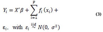
Longitudinal data, which involves collecting repeated measures from multiple subjects over time, is common in various scientific fields such as biology, ecology, and clinical research. Parametric mixed-effects models are robust and effective tools that are widely used for modeling the correlations and variations within and between subjects in longitudinal data when the models are correctly specified. These models are well-established, concise, and efficient, and have been extensively studied and developed [25-28]. However, as mentioned above, parametric models can be limiting and vulnerable to errors arising from assumptions made during the modeling process. This is particularly evident when modeling a repeated outcome variable as a function of time and other covariates, where the time effect can be too complex to be accurately captured under a parametric model. To overcome these limitations, nonparametric models have been developed for analyzing longitudinal data, which can be more flexible in relaxing the assumptions made by parametric models, but these models tend to be more complex [44]. Semiparametric Mixed-effects Models (SMMs) offer a balanced approach to longitudinal data analysis by integrating the advantages of mixed-effects modeling with the flexibility of nonparametric regression [1]. Detailed discussions of SMMs can be found in various sources [40, 45].
Suppose that yij(i = 1,…,n;j = 1,…,ni) is the response for the ith subject at time point tij, the SMM can be expressed as follows:
 (6)
(6)
where the variable β is a p × 1 vector of coefficients associated with covariates xij, and fi(·) refers to twice-differentiable smooth functions of time or nonparametric fixed effects. bi includes independent q × 1 vectors of random effects’ coefficients associated with covariates zij. Ui(·) is an independent and smooth random-effects process, and εij is an independent measurement error that occurs at a time tij, which cannot be explained by either the fixed-effects component (x’ijβ + ∑ip=1fi(xi)) or the random-effects component (z’ijbi + ∑ip=1Ui(xi)) [46]. In general, SMMs consist of four major components: parametric fixed-effects (x’ijβ), nonparametric fixed-effects (fi(·)), parametric random-effects (z’ijbi), and nonparametric random-effects (Ui(·)). In their work, Wu and Zhang [47] presented a comprehensive analysis of various types of semiparametric mixed-effects models by examining different scenarios where one or two components of the model (expressed in equation (6)) are dropped. For instance, if the nonparametric random-effects component is removed from SMM (6), the resulting model is expressed as equation (7) below, which is equivalent to incorporating the random-effects into the additive model (3), known as the additive mixed model (AMM):
 (7)
(7)
where X’, β, fi(·), zij, bi, and εij are defined as in (3) and (6); εij~N(0,R) and bi~N(0,Gθ). Both covariate matrix R and Gθ are positive-definite matrices depending on a parsimonious set of covariate parameters [32, 34, 40]. The AMM expressed in equation (7) can be thought of as a combination or hybrid of linear mixed models and additive models [48, 49].
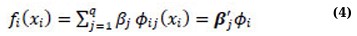
Generalized additive mixed models (GAMMs) are an extension of the AMM that allow the response variable to have a distribution other than the Gaussian [32, 48, 49]. A GAMM is a more complex and flexible model than an LMM, where a portion of the linear predictor is specified as a sum of smooth functions of one or more predictor variables, and non-normally distributed outcomes are included [29, 32, 37, 48, 49]. Therefore, GAMMs can be considered as an additive extension of generalized linear mixed models (GLMMs) [32, 34, 37, 48].
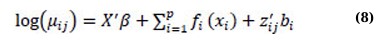
In a previous study, Yirga et al. [4] discussed a negative binomial mixed-effects model. This model specifies the expected CD4 count using the mean µij and parameter θ, which regulates over-dispersion. The relationship between the count response’s conditional mean and the linear predictors is established through the logarithmic link function. Consistent with our earlier work by Yirga et al. [4], this study employs an additive negative binomial mixed-effects model, in which some or all linear terms are replaced with more flexible functional forms. The model can be expressed as follows:
 (8)
(8)
where again, each fi(·) is an unspecified smooth function. The model’s flexibility expressed in Eq. (8) is increased by using a nonparametric form for the functions fi(·), but the additivity is still maintained, making it possible to interpret the model similarly to the GLMM form. One of the examples of a GAMM is the additive negative binomial mixed-effects model [48].
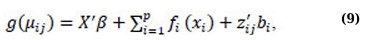
The general structure of GAMM can be expressed in the following way:
 (9)
(9)
where yij is a non-normally distributed outcome, fi(·) is a centered twice-differentiable smooth function, g(·) is a monotonic, differentiable link function, and X’, β, zij, bi, and εij are defined as in equations (3) and (6). To make statistical inference for GAMM, the nonparametric function fi(·) must be inferred, which involves the estimation of smoothening parameters and variance components. When the response is Gaussian, and the link function is identity, Restricted Maximum Likelihood (REML) is used to estimate the nonparametric functions, smoothers, and variance components in GAMM [50, 51]. On the other hand, Penalized Quasi-Likelihood (PQL) is commonly used to estimate the parametric and nonparametric functions in GAMM when the response is non-Gaussian [29]. A detailed discussion of PQL and other approaches to estimate smoothing parameters and variance components in GAMM is also available and can be found in several literature sources [29, 41, 44, 49].
3. RESULTS
Tables 1 and 2 provide a summary of the baseline characteristics for the study. The study involved 235 participants who were observed multiple times, ranging from 2 to 61 times, with a median equal to 29, resulting in a total of 7019 observations. Out of the total 7019 observations, the response variable (CD4 cell count) has 1.5% missing observations. Given the very low proportion of missing data (<5%) and the consistency of results across approaches [4], we proceeded with complete-case analysis in the present study. Of the total participants, 105 women were living in the rural area of Vulindlela [5], which represents 44.7% of the participants, while 130 women (55.3%) lived in the urban area of eThekwini (Durban, KwaZulu-Natal, South Africa) [5]. Participants enrolled in the study were between 18 and 59 years old, with an average age of 27.15 years and a standard deviation of 6.56 years. The CD4 count and viral load at enrollment had an average of 570, with a range of 182 to 1575 and a standard deviation of 229.6, and 140442.31, with a range of 1 (undetected) to 5510000 and a standard deviation of 454895.893, respectively. Furthermore, the participants' average Body Mass Index (BMI) at enrollment was 28.93, ranging from 17.89 to 54.89, with a standard deviation of 7.4. Of the participants, 182 women (77.4%) reported having a stable relationship, and 224 (95.3%) completed secondary education. A majority of the participants (78.8%) identified themselves as sex workers, according to their self-reporting and previous studies [1, 4, 18].
Building on the earlier work conducted by Yirga et al. [4], which employed a parametric negative binomial mixed-effects model (NBMM) within the GLMM framework, assuming a linear relationship between the outcome and covariate, this study extends the approach by incorporating nonparametric modeling. Specifically, this study utilizes a Generalized Additive Mixed Model (GAMM) to capture nonlinear effects of time, age, and baseline BMI, while retaining a parametric specification for the remaining covariates. Eqs. (10a) and (10b) represents the proposed model:
 (10a)
(10a)
 (10b)
(10b)
| Variable | Descriptive Measures | |||
|---|---|---|---|---|
| Mean | Standard Deviation | Minimum | Maximum | |
| CD4 cell counts (cells/µL) | 570 | 229.6 | 182 | 1575 |
| HIV viral load (cells/µL) | 140442.31 | 454895.893 | 1 (undetected) | 5510000 |
| Age (Years) | 27.15 | 6.56 | 18 | 59 |
| Body Mass Index | 28.93 | 7.4 | 17.89 | 54.89 |
| Variable | Total | Variable | Total |
|---|---|---|---|
| Place of Residence | Number of Sexual Partners | ||
| Rural | 105 (44.7%) | No partner | 43 (18.3%) |
| Urban | 130 (55.3%) | Stable partner | 182 (77.4%) |
| Educational Level | Many partners | 10 (4.3%) | |
| Primary schools | 11 (4.7%) | Number of Women | 235 |
| Secondary schools | 224 (95.3%) | ||
Here, yij denotes the vector of the response variable representing CD4 cell counts, g(·) is the log link function, and the outcome follows a negative binomial distribution with mean = µij and variance = µij + θµij2. The terms γi represent parametric regression coefficients, fi(xij) are smooth, nonparametric functions of the covariates X, and the random effects bi are assumed to follow a normal distribution with mean zero and covariance matrix Gθ, denoted as bi~N(0,Gθ) [1, 29, 32, 34, 40].
The proposed model (10) was fitted using the R package mgcv with the gamm command [52]. The gamm command is designed to avoid overfitting by penalizing excessively ‘wiggly’ lines, so it is possible to apply this penalty to all continuous covariates within smoothing functions. The model assesses the level of support for a ‘wiggly’ shape based on the data [31]. Additionally, there are multiple options available for controlling model smoothness with splines. Model (10b) was fitted using thin-plate (tp) shrinkage splines in the R package mgcv, and convergence was achieved. Thin plate shrinkage splines have certain advantages, such as not requiring knot selection and providing efficient, stable approximations. They can also be constructed for smooths of multiple covariates simultaneously [53]. Furthermore, the shrinkage smoothers obtained through the use of the ‘bs’ option within the ‘s’ command are designed in a way that allows them to be penalized and ultimately excluded from the model entirely, resulting in smooth terms that do not contribute to the model [37, 48]. The model output consists of two parts: a parametric component and a smooth (nonparametric) component. The smoother coefficients (represented by γi’s) are embedded within the smoothers and are generally difficult to interpret. To fit a smoother for a specific predictor, the ‘s’ function can be utilized within the ‘gamm’ command [52]. The degree of smoothing in a smoother is quantified by the effective degrees of freedom (edf), which provide information on the curvature of the fitted line. A relatively high edf value (≥ 8) suggests that the curve is highly non-linear, while a smoother with an edf of 1 indicates that the relationship with the outcome is linear [31, 48].
Using the proposed additive negative binomial mixed-effects model (model (10)), Table 3 displays the logarithm of the expected CD4 count in the form of parameter coefficients and the approximate significance of the smooth terms. The table indicates that the baseline viral load and initiation of HAART have a significant impact on the progression of patients’ CD4 count. The ‘parametric coefficients’ section reveals that the patients’ viral load at the baseline has an unfavorable effect on the log of expected CD4 count, even with minimal changes in units. In addition, the expected number of CD4 cells for a patient who initiates HAART increases by 1.233 (e0.2092) units (95% CI: 1.851e-01 to 2.333e-01) in comparison to pre-HAART initiation, while other variables are kept constant. To improve clinical interpretability, the effect of baseline viral load was rescaled to reflect a 1-log10 increase. A one-log10 higher viral load was associated with an estimated 1.58 × 10⁻⁶ decrease in expected CD4 count (95% CI: −2.50 × 10⁻⁶ to −6.58 × 10⁻⁷).
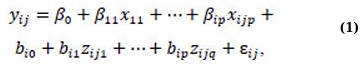
The results of edf from Table 3 indicate that age (edf = 14.24, p-value < 2e-16) and time (edf = 10.343, p-value < 2e-16) variables have a notably significant non-linear effect on the CD4 count of patients. The level of spline for baseline BMI (edf = 3.044, p-value = 2.21e-06) shows a significant non-linear relationship with the response variable. Figure 1 depicts the fitted penalized spline plots obtained from the analysis, with the shaded area representing the approximate 95% confidence bands at each point. The y-axis displays the effect of the smooth term, with ‘s’ denoting the smooth term and the number in the parentheses indicating the corresponding smooth term’s edf value [34]. Upon visual inspection of (Fig. 1), it is apparent that the overall shape of the smoothers indicates a higher progression of CD4 counts over time. The increment rate is observed to be low for the initial four years (48 months) and then gradually increases. An increase in CD4 count over time may provide evidence of long-term benefits of HAART. The smooth terms age and baseline BMI also show similar relationships, with older patients and those with higher BMI at enrollment having a higher CD4 count.
| Parameter Coefficients | Estimate | Std. Error | t-value | 95% CI of the Estimate | p-value |
|---|---|---|---|---|---|
| Intercept | 6.334e+00 | 1.172e-01 | 54.053 | (6.104e+00, 6.564e+00) | < 2e-16 |
| Baseline viral load | -1.581e-07 | 4.709e-08 | -3.358 | (-2.504e-07, -6.582e-08) |
0.00079 |
| Educational level (ref.= Primary school) | |||||
| Secondary school | -1.500e-01 | 1.056e-01 | -1.420 | (-3.570e-01, 5.703e-02) | 0.15564 |
| HAART initiation (ref.= Pre HAART initiation) | |||||
| Post HAART initiation | 2.092e-01 | 1.229e-02 | 17.021 | (1.851e-01, 2.333e-01) | < 2e-16 |
| Place of residence (ref.= Rural) | |||||
| Urban | 3.569e-02 | 4.367e-02 | 0.817 | (-4.989e-02, 1.213e-01) | 0.41375 |
| Number of sexual partners (ref.= No partner) | |||||
| Stable partner | 4.490e-02 | 5.529e-02 | 0.812 | (-6.347e-02, 1.533e-01) | 0.41679 |
| Many partner | -6.587e-02 | 1.116e-01 | -0.590 | (-2.847e-01, 1.529e-01) | 0.55521 |
| Approximate Significance of Smooth Terms | |||||
| Smooth Terms | edf | Ref.df | F-value | p-value | |
| s(Age) | 14.124 | 14.124 | 4.710 | < 2e-16 | |
| s(Time in months) | 10.343 | 10.343 | 37.692 | < 2e-16 | |
| s(Baseline BMI) | 3.044 | 3.044 | 9.759 | 2.21e-06 | |
Estimated smooth curve for the GAMM model containing all smooth terms [1].
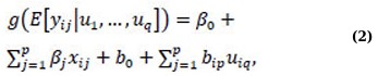
Diagnostic plots for checking the adequacy of the fitted model [1].
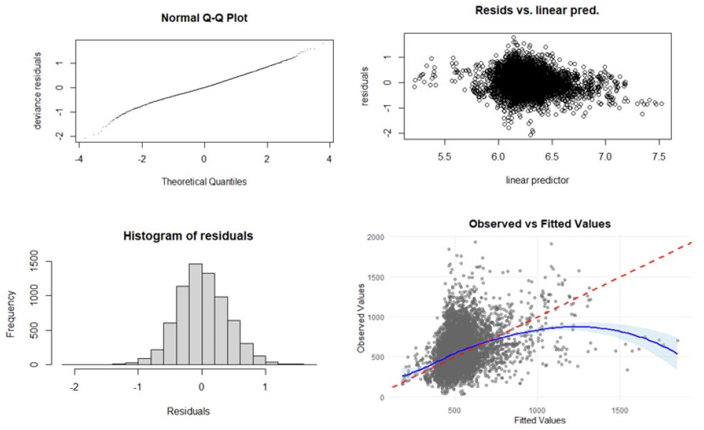
To validate the fitted model, model diagnostic graphs were plotted and presented in Fig. (2). The normal Quantile-Quantile (Q-Q) plot on the upper left is almost straight, indicating that the distributional assumption is reasonable. The histogram of residuals, shown on the lower left, is approximately Gaussian. The residual plot versus the fitted values (linear predictor) in the upper right reveals that the variance is approximately constant as the mean increases. In general, the observed values are positively correlated with the fitted values, as demonstrated in the lower right plot of Fig. (2). However, the blue smooth trend curve deviating considerably from the red reference line (perfect prediction) at extremely high values indicates systematic underprediction, increasing variance heterogeneity across the prediction range. Future studies should explore variance modeling structures and potential transformations to improve model performance across the full range of CD4 count values. Influential observations with extremely high values may be worth investigating.
4. DISCUSSION
It is assumed in multiple linear regression that the link between the outcome variable (Y) and the predictors (X) remains linear or monotonic across all values. However, not all regressions need to be linear or have a specific structure, such as being monotonic. To some extent, this issue can be addressed by using polynomials [54, 55]. However, polynomials may not always be desirable in terms of the model’s fit properties because adding more powers of the covariate (X) can create a model selection problem. Moreover, increasing the number of powers of the covariate (X) in the polynomial model may not always improve the model's accuracy [56] and could lead to a Runge phenomenon, which is the problem of oscillation at the edges of an interval when using high-degree polynomial interpolation points. Nonparametric regression methods, like Locally Weighted Scatterplot Smoothing, also known as the LOESS smoother, may be a better option for generalization, since this method imposes no restrictions on the functional form between the outcome and the covariates, except that it requires smoothness. This implies that if there are no restrictions, the fits will be more computationally intensive. However, if LOESS smoothers are correctly applied, they provide additional information from the data; however, the information we obtain depends on the selection of the smoothing parameter, as is the case with kernel smoothing. GAMs provide a solution to these problems by offering a framework for modeling flexible, nonlinear relationships in the data.
GAM extends both multiple linear regression models and GLMs, enabling the modeling of outcomes from the exponential family, including continuous, discrete, count, and proportion data. GAMs offer flexibility and are used to better understand and analyze complex, nonlinear relationships within data. They effectively characterize key features of the relationship between the response variable and the covariates by using smooth functions, such as splines, which allow for a broad range of functional forms [1]. To fit a GAM, one can use the gam function from the mgcv package in R. When fitting a GAM, the covariate (X) needs to be included in the s (smooth) function to specify a flexible relationship. The flexibility of splines allows GAM to capture various nonlinear aspects [1]. The flexible smooths in GAMs are made of many smaller functions called basis functions. Each smoother is the sum of several basis functions, and each basis function is multiplied by a coefficient, which is a parameter in the model. With GAMs, it is possible to include a mixture of smooth, linear effects, continuous, counts, or categorical variables in a multiple regression model format. Not all terms in a GAM have to be nonlinear, as it is possible to combine linear and nonlinear terms. Adding a linear term does not require repelling the predictor term in the s function. Linear terms are particularly useful when we have categorical variables as predictors in the GAM [1].
GAMM, a mixed-effects version of GAM, is the most effective model for analyzing nonlinear trajectories in longitudinal data [1]. The relationship between the outcome variable and the predictors is often complex and involves unknown functional forms of covariates, making parametric models inflexible. As a result, this study utilized the generalized additive mixed-effects approach. For the analysis of the longitudinal CD4 count of HIV-infected patients, this study utilized an additive negative binomial mixed-effects model, which is an example of a GAMM. The model accounted for non-parametric effects of time, age, and baseline BMI, as well as parametric effects of some available covariates. The analysis identified that HAART initiation was significantly associated with higher CD4 counts over time, while higher baseline viral load was significantly associated with lower CD4 count over time, consistent with established clinical understanding. The analysis also revealed a significant nonlinear effect involving age, baseline BMI, and time. The nonparametric component indicated that older participants (above 40 years) tended to have higher progression of CD4 count, and individuals with higher baseline BMI showed patterns of CD4 improvement over follow-up. However, this does not imply that patients with higher BMI should be neglected clinically. Instead, the study suggests that BMI plays a role in drug metabolism and can influence the progression and immunological responses of HAART [1, 57, 58]. The findings may reflect underlying physiological or metabolic factors, although such interpretations remain speculative and cannot be confirmed by this observational analysis.
The significant nonlinear effect of time suggested that CD4 counts increased gradually and only began to rise more noticeably after several follow-up visits. Therefore, the study emphasizes the importance of initiating effective HAART immediately after HIV infection is confirmed to suppress the increase of viral loads and induce potential ART benefits that accumulate over time. HIV patients who are not stable on HAART may be at higher risk of developing illness if infected with OIs [1]. Viral load rebound due to inconsistent ART use is a major concern in HIV management. However, these findings should be interpreted with caution, as the study was not designed to assess underlying causal mechanisms. All interpretations reflect main effects only, as no interaction terms with HAART or between covariates were included in the model. The nonlinear associations observed for age, baseline BMI, and time reflect overall patterns in CD4 count trajectories and should not be interpreted as modifying the effect of HAART, as no interaction terms were included in the model. Any potential treatment-modifying effects remain speculative and would require explicit interaction modeling in future analyses.
Moreover, the CAPRISA 002 cohort consists of high-risk South African women, many of whom were sex workers, representing a population that differs significantly from other groups, such as men, lower-risk women, or individuals from different geographic or socioeconomic settings. It must be noted that CD4 trajectories, treatment access, and underlying health conditions may vary across populations; therefore, the external validity of our findings is limited, and causality cannot be inferred from this study. The associations observed reflect patterns within this specific cohort and may be influenced by unmeasured confounding, selection processes, measurement limitations, differential follow-up, or other cohort-specific factors. The observational design, potential selection bias at enrollment, differential loss to follow-up, and measurement variability, such as the timing of CD4 and viral load assessments, may affect the interpretation of estimated results. Therefore, the interpretation of these findings requires appropriate caution.
5. LIMITATIONS OF THE STUDY
This study has several important limitations that should be considered when interpreting the findings. The analysis is based on an observational cohort, which limits the ability to draw causal inferences about the relationships between HAART initiation, viral load, demographic factors, and CD4 count trajectories. Unmeasured confounding, selection processes, and time-dependent biases may influence the observed associations. Additionally, the data were collected during a historical period when ART eligibility criteria and treatment guidelines differed from current standards, which may affect the applicability of the findings to contemporary clinical contexts.
Moreover, no formal power calculation was conducted for this secondary analysis, and the study may be underpowered to detect subtle nonlinear effects or interactions. Even though the cohort included repeated CD4 measurements, follow-up was unbalanced, with participants contributing 2 to 61 observations. Irregular visit spacing and differential loss to follow-up may introduce informative censoring or survivorship bias. While the mixed-effects modeling framework accommodates unbalanced data, residual bias cannot be fully excluded.
Although model diagnostic plots generally support the adequacy of the fitted model, certain limitations warrant further investigation. Notably, the observed-versus-fitted values plot indicates systematic underprediction at extreme values, suggesting increasing heterogeneity in variance across the prediction range. This pattern may reduce model accuracy in the upper tail and suggests potential instability driven by influential observations with unusually high CD4 values, which may reflect biological variability or measurement inconsistencies not fully accounted for by the current model.
To improve model performance, future studies should explore more flexible variance structures, such as heteroscedastic models or appropriate data transformations, to better capture the full range of CD4 counts. Influence diagnostics were conducted in a previous study by Yirga et al [5], which may inform strategies to mitigate the effect of extreme observations in future analyses. These refinements would enhance predictive reliability and offer deeper insights into CD4 progression under HAART, especially for patients with unusual immunological responses.
Together, these limitations highlight the need for cautious interpretation of the findings and underscore the value of future studies incorporating causal inference methods, updated cohorts, and more flexible modeling frameworks.
CONCLUSION
This study employed an additive negative binomial mixed-effects model to investigate the progression of CD4 cell counts among HIV-infected participants, incorporating both parametric and nonparametric covariates. The results indicate that baseline viral load and HAART initiation were significantly associated with patterns of CD4 count over time. Higher baseline viral load was associated with lower expected CD4 levels, whereas HAART initiation yielded a substantial increase in CD4 count, highlighting its treatment benefit.
The nonparametric components of the model revealed pronounced nonlinear effects of time, age, and baseline BMI. The edf and corresponding p-values indicated that these variables demonstrated statistically significant and complex influences on CD4 progression. Notably, CD4 counts increased gradually over follow-up, with a more pronounced rise after approximately 4 years, suggesting long-term immunological benefits of sustained HAART; however, this pattern should be interpreted as descriptive rather than causal. Additionally, older age and higher baseline BMI were positively associated with improvements in CD4 count, potentially reflecting underlying physiological factors such as drug metabolism and immune responsiveness.
These findings reinforce the importance of timely and consistent initiation of HAART following HIV exposure to mitigate viral load and optimize long-term immunological outcomes. The observed nonlinear dynamics further emphasize the need for individualized treatment strategies that account for patient-specific characteristics, including age and BMI. Moreover, the potential for viral load rebound due to inconsistent ART use remains a critical concern in HIV management, underscoring the necessity of adherence support and ongoing clinical monitoring. Overall, the findings describe patterns of CD4 evolution in this cohort and should not be interpreted as clinical recommendations. Future work incorporating causal inference methods or survival/competing-risk frameworks may help clarify the mechanisms underlying these associations.
Survival data analysis is a statistical method used to analyze data in which the variable of interest is the time until a certain event occurs [59]. This is also known as competing risk analysis when there are multiple events. The concept of competing risks is based on the idea that individuals are exposed to several hazards that can cause an event or experience multiple types of the same event (competing events), which will be addressed in future research.
AUTHORS’ CONTRIBUTIONS
The authors confirm contribution to the paper as follows: A.A.Y.: Responsible for acquiring the data, conducting the analysis, and writing the manuscript; A.A.Y., H.G.M., M.M., T.B., S.F.M., and D.G.A.: Collaborated in defining the research question. All authors reviewed and discussed the findings and provided feedback at all stages of the manuscript preparation. All authors contributed extensively to the work presented in this paper. All authors read and approved the final version of the manuscript.
LIST OF ABBREVIATIONS
| CAPRISA | = Centre of the AIDS Programme of Research in South Africa |
| GLM | = Generalized Linear Model |
| LMM | = Linear Mixed Model |
| GLMM | = Generalized Linear Mixed Model |
| AM | = Additive Model |
| GAM | = Generalized Additive Model |
| SMM | = Semiparametric Mixed Model |
| GAMM | = Generalized Additive Mixed Model |
| CD4 | = Cluster of Differentiation 4 Cell (T-Lymphocyte Cell) |
| VL | = Viral Load refers to the number of hiv copies in a milliliter of blood (Copies/Ml). |
ETHICAL STATEMENT
Ethical approval for this study was obtained from the Research Ethics Committee of the University of KwaZulu-Natal (E013/04), the University of the Witwatersrand (MM040202), and the University of Cape Town, South Africa (025/2004).
AVAILABILITY OF DATA AND MATERIALS
The data of current study are available from corresponding author, [D.A], on a reasonable request.
FUNDING
This study did not receive direct funding or grant support. As part of the first author’s postdoctoral research program, the first author received support from the Data Science Initiative for Africa (DSI-A) programme, the University of KwaZulu-Natal, Harvard T.H. Chan School of Public Health (HSPH), and Heidelberg Institute of Global Health (HIGH). The DSI-Africa programme is supported by the Fogarty International Center of the National Institutes of Health under Award Number U2RTW012140. The content is solely the responsibility of the authors and does not necessarily represent the official views of the National Institutes of Health.
CONFLICT OF INTEREST
Dawit Ayele and Sileshi Melesse are the Editorial Advisory Board members of The Open Public Health Journal.
ACKNOWLEDGEMENTS
We express our gratitude to CAPRISA for providing us with access to the data from the CAPRISA 002: Acute Infection Study. CAPRISA is funded by the National Institute of Allergy and Infectious Diseases (NIAID), National Institutes of Health (NIH), and U.S. Department of Health and Human Services (grant: AI51794). The authors would like to extend their gratitude to Dr. Nonhlanhla Yende-Zuma, who is the head of the Biostatistics unit at CAPRISA, for her cooperation, assistance, and technical support.
DISCLOSURE
Portions of this manuscript were previously published as part of the first author’s doctoral dissertation. The dissertation titled “Statistical Modeling of Acute HIV Infection from a Cohort of High-risk Individuals in South Africa” was submitted in partial fulfillment of the requirements for the PhD degree and is publicly available through the University of KwaZulu-Natal’s repository: https://researchspace.ukzn.ac.za/home. The current manuscript includes revised and expanded content that has not been previously published in a peer-reviewed journal.